How LLMs work
A deep dive into the internals of Large Language Models (LLMs). Understanding how LLMs work helps us understand both their power and their limitations.

Introduction
For many, AI is synonymous with chatbots like Claude, ChatGPT, or Gemini. These are powered by Large Language Models (LLMs), and understanding how they work helps us appreciate their power and their limitations. I’ll describe here the key building blocks and how they come together.
Many know that LLMs work by predicting the next token in a sequence, but this explanation is hard to square with experience. The richness of their output is a product of clever design and immense scale, and in this article we’ll uncover what goes into creating it.
This article explains how LLMs work from the ground up. Given their impressive abilities, the architecture is relatively straightforward compared to many software systems. Their power comes from scale, not complex design, with more than a trillion parameters in the largest models.
But this is still a big topic and this article is correspondingly long. The aim is for it to be understandable by a general technical audience with no background in AI or machine learning.
The article opens with a summary of the key points. Parts 1 and 2 focus on building conceptual understanding. Part 1 covers inference: how a model generates output. Part 2 covers training: how the weights get their values. Part 3 goes much deeper into real-world practicalities, optimisations, and edge cases. You can skip Part 3 and go straight to the recap and conclusion if you prefer. The appendices provide background on topics kept brief in the main text: mathematical models, neural networks, and matrix multiplication.
Notes:
- I have included some maths that is fairly simple but perhaps unfamiliar. You can safely skip over these sections and still gain a good understanding.
- This is my attempt to play back what I have learned, but I’m not a specialist. Interestingly, the MSc in Neural Networks I got 25 years ago is still somewhat relevant, but much is also new.
Summary
This article expands on the following points:
- LLMs generate output one token at a time. Each token is produced by looking at previous context, with no lookahead.
- The fluency, knowledge, and apparent reasoning all emerge from patterns the model has learned. Training on huge bodies of text lets the model learn the structure of language, the knowledge encoded in it, and patterns of reasoning that appear in human-written text.
- Pre-training teaches the model to predict the next token across a vast corpus (body of text). Post-training shapes it into an assistant: following instructions, declining harmful requests, and using tools.
- LLMs have no memory between conversations and no access to the world unless given tools.
- The attention mechanism is how the model makes use of context: at each layer, every token pulls relevant information from preceding tokens. Attention is causal: each token only ever looks backwards, which is what makes left-to-right generation possible.
- Feed-forward layers act like a pattern-retrieval memory: recognising what the model is processing and contributing relevant knowledge encoded during training.
- Stacking these two operations across dozens of layers is what produces the richness of the output. There is no single place where “understanding” happens; it is distributed across the whole network.
- Limitations follow directly from the architecture: the model can produce confident-sounding text that is wrong, struggles with tasks that require exact symbol manipulation such as arithmetic, and is bounded by what was in its training data. Output is probabilistic, not deterministic.
- Making the model bigger increases its knowledge but has less effect on its reasoning ability. Extensive post-training and extended reasoning (“thinking mode”) are the most effective ways discovered so far to boost reasoning.
- Some limitations of LLMs are inherent and will only be fixable by combining them with other mechanisms.
Part 1: Inference
Overview
LLMs are mathematical models built from a small number of repeated components. Before diving into each one, it helps to see how they connect. (See Appendix 1 for an explanation of what a mathematical model is.)
In operation, an LLM takes as input a sequence of tokens, and outputs its best guess at which token should come next. This happens one token at a time: each new token is appended to the context and the process repeats, producing fluent text word by word. This process is called inference.
In this part and Part 2, we’ll focus on what are called pure transformer models as they give a useful starting point for building a conceptual understanding. Part 3 touches on alternative model architectures.
Internally, these transformer models process input by following the steps below once for each token generated. Each is explained in subsequent sections.

- Each token in the input is converted to a token ID and then to an embedding vector: a list of numbers that are a semantic representation of the token.
- This embedding vector is used as the initial value of the residual stream for each token, which is passed through a few dozen layers that are identical in structure, with separately learned weights. Each layer has two sublayers:
- an attention sublayer lets each token draw information from preceding tokens in the sequence;
- a feed-forward sublayer processes each token independently through a small neural network to add relevant information.
- At each sublayer, the output is added to the residual stream, enriching it.
- After the final layer, the last position in the residual stream is used to predict the next token.
The parameters that get learned during training are:
- the transformations that convert text to embeddings;
- the weights inside the attention and feed-forward sublayers, learned separately for each layer;
- the transformation that converts the last layer’s final residual stream into a prediction of the next token.
The weights are fixed once training is complete. The model does not learn from individual conversations: nothing said in a chat session updates the underlying parameters.
Converting text to tokens
LLMs do not process text character by character or word by word. Instead, text is split into tokens: chunks that are roughly syllable- to word-sized.
The most common approach is byte pair encoding (BPE), which starts with individual characters and repeatedly merges the most frequent adjacent pairs until a target vocabulary size is reached (up to 200,000 tokens for current frontier models). Common words end up as a single token; rarer words get split into pieces. For example, the word “tokenisation” might be split into [token, isa, tion], while “cat” would be a single token. Numbers, punctuation, and whitespace are also tokenised, and tokens often include a leading space to signal word boundaries. The merge rules themselves are learned from a corpus by frequency, but this happens once, before model training, and the tokeniser is then frozen. Applying it to split text is deterministic, and the tokeniser is considered separate from the LLM itself.
The model sees a sequence of tokens, not characters or words. Unusual spellings, made-up words, or heavily technical text may tokenise poorly, producing many fragments that the model has seen less of during training. Arithmetic can go wrong at the tokenisation stage: “1234” may be one token, but “12345” might split differently, and the model has no direct access to individual digits.
An LLM’s context window is the maximum number of tokens it can process at once, including inputs and outputs. As a rough guide, 100 tokens corresponds to around 75 English words. Current frontier models support up to 2,000,000 token windows, meaning entire books or codebases can fit in a single context. The vocabulary (the full list of tokens the model knows) is fixed at training time. Each token is assigned a unique integer ID, and it is these IDs that flow into the next stage.
Converting tokens to embedding vectors
A token ID on its own is just an integer. The model needs a richer representation that captures what the token means, not just which entry in the vocabulary it corresponds to.
This representation is called an embedding vector. Its elements together encode the token’s meaning, but no single element maps neatly to one human-readable property. The way tokens are converted to embeddings is learned during training and is unique to each model. Tokens that appear in similar contexts end up with similar embeddings. These can be pictured as vectors in a high-dimensional space, typically 7,000–16,000 dimensions. Meaning is carried by directions through this space rather than by individual axes, and the model packs in far more distinct features than it has dimensions.
The geometry of the embedding space carries meaning: vectors for “king” and “queen” are closer to each other than either is to “bicycle.” This is what allows the model to generalise across related words and concepts. Individual dimensions are mostly not interpretable on their own; what a direction in the space means is fixed entirely by training. Researchers can “probe” embeddings to recover some of this structure, but the opacity doesn’t matter in practice: these embeddings are just part of the model’s internal machinery, not something we ever need to read directly.
In practice, this conversion is done with an embedding table: a large matrix with one row per token in the vocabulary. Each row is the vector of numbers that represents that token’s embedding. Looking up a token’s embedding is simply selecting the relevant row from this table.
At this stage, the embeddings contain no information about position. “the cat sat” and “sat the cat” would produce identical embeddings for each token, which is a problem for any task where word order matters. To solve this, positional information is added to each vector. See Encoding token position for more detail.
The result is a sequence of vectors, one per input token, each encoding the token’s meaning and position. This sequence is what enters the first layer of the model.

Residual stream
As the input passes through the model, each token carries a vector that starts as its embedding and is progressively refined at every layer, adding context and interpretation. This vector is called the residual stream.
Each token has its own residual stream. Across many layers, each token’s vector is gradually shifted from a representation of what that token is toward a prediction of what the next token should be. At inference time, only the last residual stream vector in the final layer is used to predict the next token. But all tokens are processed at every layer because later layers’ attention depends on what earlier layers produced for every position, not just the last one.
Before each sublayer, the residual stream is normalised: rescaled so its values sit within a predictable range, like adjusting the volume on different audio tracks so none drowns out the others. This keeps the values at a consistent scale as they pass through dozens of layers. Without it, values can grow or shrink exponentially during training, making the model impossible to optimise reliably.
Attention layers
Attention is the mechanism that lets each token query preceding tokens in the sequence and pull in relevant information. This is what allows the model to resolve references (in “the dog chased the cat because it was hungry,” “it” refers to the dog), track long-range dependencies, and build up a contextualised understanding of each token.
Causal attention
Each token only attends to tokens that came before it in the sequence. This is called causal (or masked) attention. It is what makes left-to-right generation possible. Because each token only looks backwards, you can generate one token at a time, append it to the sequence, and immediately run the process again.
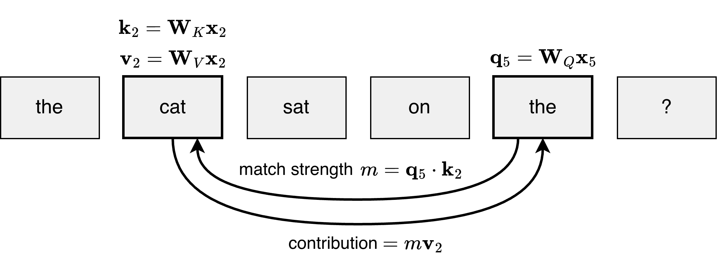
For each token, the attention mechanism asks how relevant each of the preceding tokens is to understanding this one.

To calculate the contribution of a given preceding token to understanding the token of interest:
- The later token “queries” the earlier token to determine how relevant it is. This is done by comparing the later token’s “query” vector to the earlier token’s “key” vector to produce an attention score. This is described more below.
- The contribution is calculated by multiplying the earlier token’s “value” vector by the attention score.
Query, key, value
Each token produces three vectors that govern how it takes part in attention: a query, a key, and a value.
- The query vector represents what kind of information the token is looking for from previous tokens, e.g. the gender of a pronoun depends on the gender of the subject it refers to.
- The key vector represents what kind of information it has to offer future tokens, e.g. a subject would advertise that it has gender information.
- The value vector represents the actual information it will contribute if selected, e.g. a subject would specify which gender it is.
Queries are matched against keys to decide what each token attends to, and the values of the chosen tokens are what it draws in.
Each vector is a linear transformation of the token’s normalised residual stream vector , using a set of learned matrices:
See Appendix 3 for an explanation of matrix multiplication and an illustration of the linear transformations that matrices can encode.
Each layer has its own set of transformation matrices , , and .
The query and key vectors must have the same dimensionality (written ) so that their dot product can be calculated. Most models also have value vectors of the same size.
Calculating the contribution
To decide how much attention token should pay to token , the query of (vector ) is compared to the key of (vector ) by calculating the dot product (), which is a measure of how similar they are. This produces a score for how relevant is to .
Output
The attention scores are passed through the softmax function, turning them into attention weights. For each query token, those weights run across the tokens it attends to and sum to 1, so they act like proportions: how much of the token’s attention goes to each of the others. Softmax also sharpens the distribution, boosting the highest-scoring tokens and shrinking the rest.
The result is that a token attends heavily to the tokens that scored highest against its query, and barely at all to the rest. That selectivity lets each token pull in just the context relevant to it, such as a pronoun drawing on its antecedent or a verb on its subject.
The output for each token is then the weighted sum of all the preceding tokens’ value vectors, using these attention weights.
This output is added back into the residual stream and passed to the feed-forward sublayer.
Mathematical detail
In full, the contribution to residual stream is:
The subscript in records which index the function normalises over. Here, it’s , the position of each token being attended to. That is what makes the weights for a given query token sum to 1, normalising across the attended-to tokens rather than across the queries.
The attention scores () are divided by before applying softmax. Dot products naturally grow larger as increases, because they sum more terms. Without this correction, softmax becomes so sharp that attention collapses to a single token: the weights stop responding to changes in the scores, and the model can no longer adjust which tokens attend to which during training.
The KV cache
Generation produces one token at a time, and each step requires running attention over the full sequence so far. Naively, this would mean recomputing the key and value vectors for every earlier token at every step.
But those key and value vectors don’t change. At a given layer, a token’s key and value depend only on its own residual stream at that layer, which was fixed the moment that token was processed. Only the new token’s query, key and value are genuinely new at each step.
The KV cache uses this property to avoid recalculating attention for every forward pass (one complete run of the input through all the model’s layers). Each layer stores the key and value vectors it has already computed, and at each generation step only the new token’s key and value are added. (The query doesn’t need to be cached as it’s only used once, when generating that token’s contribution from preceding tokens.) The cache grows linearly with the number of parsed and generated tokens and is the main reason that memory consumption rises as context and output length grow.
Feed-forward layers
After the attention sublayer, each token passes independently through a simple two-layer “feed-forward” neural network. The name comes from the idea of feeding information through to the next layer of the network and doesn’t refer to the token sequence. There is no communication between tokens here: each token’s residual stream vector is processed on its own. (See Appendix 2: Neural networks for more background on the internals of such a network).
The feed-forward sublayer takes the residual stream for one token and projects it into a much larger intermediate space, typically four times the embedding dimension. Each dimension in that larger space corresponds to a neuron, and each neuron learns to detect a particular combination of features in the incoming representation. An activation function is applied to each neuron’s output, introducing the non-linearity that allows the network to represent complex patterns. The result is then projected back down to the original embedding dimension.
The attention layer is where tokens gather information from each other and the feed-forward layer is where that information gets processed and transformed. Research into what these feed-forward layers actually compute suggests they behave somewhat like a key-value memory: recognising patterns in the current representation and retrieving associated information encoded in their weights during training. Attention adds context, while feed-forward adds information.
The feed-forward sublayers make up the bulk of a model’s parameters. In a typical dense model, they account for roughly two-thirds of the total parameter count, with the attention weights making up most of the remainder.
Predicting the next token
After the final layer, the residual stream at the last token position holds a rich representation of everything in the input that is relevant to predicting the next token. This vector is passed through an “unembedding” matrix to produce a score (called a logit) for every token in the vocabulary. The matrix is often the transpose of the original embedding matrix but in some models is learned separately.
These logits are converted to probabilities using the softmax function mentioned earlier. The result is a probability distribution over the entire vocabulary representing how likely each possible next token is, and a token is selected based on that distribution. See Token selection algorithms for more details.
Hallucination
This token-by-token generation, based purely on probabilities learned during training, explains why LLMs sometimes confidently produce wrong answers. The model has no internal truth-checker: it is optimising for a plausible continuation of the input, not for accuracy. A wrong answer stated confidently is not a malfunction, but an emergent property of the training objective.
Meaning of residual stream vector components
As discussed, the residual stream for a given token starts by being exactly the embedding vector and by the last layer represents a prediction for the next token. As mentioned, the unembedding matrix may be the transpose of the original embedding matrix, meaning the individual dimensions in the last layer represent the same properties as the original embedding. In other models the unembedding matrix is learned separately, meaning that the properties that each dimension represents in the final layer may be different to the original token embedding. In either case, the dimensions in intermediate layers may represent somewhat different properties, and probing by performing an unembedding on intermediate layers suggests this is the case.
System prompt and conversation structure
In deployment, the input to an LLM is not just the user’s message. It is a structured document assembled by the surrounding system, typically consisting of a system prompt (instructions that define the model’s persona, constraints, and capabilities), followed by the conversation history (alternating user and assistant turns), followed by the latest user message. The model has no intrinsic identity: what makes Claude sound like Claude, or ChatGPT sound like ChatGPT, is partly the weights from post-training and partly the system prompt constructed by the operator. The model cannot distinguish between these layers; it simply processes the full input as a token sequence.
Part 2: Training
The architecture described so far assumes the model already contains weights that encode knowledge, patterns of language and patterns of thought. The process that generates these properties is called training, and it splits into two stages.
Pre-training
LLMs are trained by repeatedly attempting to predict the next token in sequences drawn from a large body (or “corpus”) of text. Given a sentence like “The capital of France is”, the model must predict “Paris.” A loss function measures how wrong the prediction was, and backpropagation adjusts the weights to make the correct token more likely next time. Appendix 2 describes this process in more detail, but briefly it is a mechanism that allows these errors to flow back through every layer of the network so that individual weights can be tweaked iteratively to move the model gradually toward more correct predictions.
This loss function measures the quality of the model’s predictions and enables training. It is simple to set up and scales to arbitrary amounts of unlabelled text. Modern LLMs are trained on many trillions of tokens drawn from web crawls, books, code repositories, and scientific papers, using thousands of GPUs over weeks or months. The compute cost of a single training run for a frontier model is tens or hundreds of millions of pounds.
The model develops internal representations of facts, grammar, logic, and world knowledge, because these are the patterns most useful for predicting tokens accurately across a sufficiently large and varied corpus. Capability is a consequence of scale and objective rather than something that is explicitly programmed.
Post-training
A model trained only on next-token prediction learns to complete text, but not necessarily to be helpful, honest, or safe. Post-training adapts the base model for use as an assistant.
Supervised fine-tuning (SFT) comes first. The model is trained on curated examples of good behaviour, adjusting its weights directly against this labelled data. This teaches the model what good responses look like.
Reinforcement learning from human feedback (RLHF) builds on this. Human raters compare pairs of model outputs and indicate which they prefer. These preferences train a reward model, which is then used to fine-tune the LLM toward outputs that score more highly. Where SFT shows the model good examples, RLHF shapes its behaviour against a reward signal derived from human comparison. Variants such as direct preference optimisation (DPO) skip the separate reward model and optimise directly on the preference data.
A further direction replaces human raters with AI feedback. Rather than asking humans to compare outputs, a model is used to evaluate responses against a set of stated principles. This allows the preference signal to be generated at much larger scale without proportional increases in human labelling cost.
The result is the assistant behaviour that users experience: the model follows instructions, declines harmful requests, and responds in a helpful register. Both stages modify the weights acquired during pre-training instead of replacing them.
Agentic training
An LLM used as an agent, such as a coding assistant, needs to do more than answer questions. It must decide when to call a tool (e.g. to read or edit a file or perform a web search), interpret the result, and continue reasoning across multiple steps.
Tool use is taught during post-training. The model is fine-tuned on examples of tool calls: structured outputs that the surrounding system intercepts, executes, and feeds back as further input. The model learns to emit these calls at the right moment, read the results, and incorporate them into its next response. It is worth noting that the LLM itself remains a next-token predictor throughout. It is the scaffolding around it — the harness that runs tools, manages the loop, and decides when to stop — which creates the appearance of an agent acting in the world.
For tasks with verifiable outcomes, such as writing code that passes tests, reinforcement learning (RL) on outcomes becomes more powerful than RLHF. Instead of asking humans to judge which response is better, the training signal comes from actually running the code: did the tests pass? This approach scales naturally because it requires no human raters, and the reward signal is unambiguous.
This is also how models learn to reason more carefully, as discussed in Scaling and optimising.
Fine-tuning for a specific task
The post-training described above is carried out by the model provider and produces a general-purpose chatbot. A separate, lighter form of training lets consumers adapt that finished model to a particular domain, style, or task.
Full fine-tuning updates every weight in the model, which is effective but expensive. This process needs enough memory to train the whole model, and it produces a complete copy of the model for each task, which is impractical at frontier sizes.
Parameter-efficient fine-tuning avoids this. The most common method, LoRA (low-rank adaptation), freezes the original weights and trains a small set of additional matrices alongside them. The trick is that the changes fine-tuning makes to a large weight matrix can be approximated well by multiplying two much smaller matrices together, so instead of updating millions of values you only train the few thousand in that pair. Only these adapters are trained and stored, often well under 1% of the model’s parameters, and several can be kept for different tasks and swapped onto the same frozen base. QLoRA goes further by quantising the frozen base to 4 bits (see Quantisation), reducing memory enough to fine-tune a large model on a single GPU.
It is worth being clear about what this achieves. Fine-tuning adjusts how the model behaves: its tone, its output format, or its handling of a specialised domain. It is not the way to give the model new facts to recall: that is better served by retrieval-augmented generation, which supplies knowledge at inference time rather than baking it into the weights.
Part 3: Going deeper
Parts 1 and 2 focused on building a conceptual understanding of the core LLM components and mechanisms, but left out details that are important in the real world. This section fills in those gaps.
You can go straight to the recap and conclusion if you prefer.
Encoding token position
Early large language models encoded position by learning a separate embedding for each slot in the sequence: position 1 got one vector, position 2 got another, and so on. These position embeddings were trained jointly with the token embeddings and added to them before the first layer. It works, but the model only ever sees positions up to the length of its training sequences, which limits how well it generalises to longer inputs.
Modern models mostly use RoPE (Rotary Position Embedding) instead. Instead of adding a position vector to each token upfront, RoPE encodes position directly inside the attention mechanism, by rotating the query and key vectors by an angle that depends on their position in the sequence. What matters for attention is how much two tokens relate to each other, so encoding the angle between them, rather than their absolute positions, means the model naturally handles relative distances. This generalises much better to sequence lengths beyond those seen in training.
Embeddings for non-English languages
Because training text is heavily English-dominated, vocabularies are skewed accordingly. A given concept may map to one or two tokens in English but to many more in languages with non-Latin scripts or rich morphology, such as Arabic, Thai, or Finnish. This has two consequences: the effective context window shrinks for users writing in those languages, and the model has seen less training signal per concept, generally producing weaker results. Tokenisation efficiency is therefore not just a technical detail; it is one mechanism by which current models perform less well in languages other than English.
Multi-head attention
In Part 1, we described a single attention “head,” but richer interpretations (and so better predictions) can be achieved by having multiple heads operating in parallel. Most modern models use this approach.
In multi-head attention, the full input residual stream is fed into every head. A model might have 16 to 128 heads per layer, depending on its size. The heads aren’t manually assigned roles: starting from random initialisation, each develops its specialisation through training because that arrangement reduces loss. One head might learn to track syntactic dependencies (subject to verb), another to resolve pronoun references, and another to link related concepts across long distances.
Each head has its own query, key, and value weight matrices (, , ), which project the full residual stream down to vectors of dimension , where is the model dimension. Splitting the dimensions this way keeps total compute roughly the same as a single full-dimension attention layer, while giving the model multiple parallel views of the same input.
Each head produces an output vector of dimension , and concatenating across heads gives a vector back at the original dimension . This is then transformed by a learned output matrix before being added back to the residual stream: . The transformation lets information from any head influence any dimension of the residual stream, rather than each head being locked to its own slice of it.
Grouping for efficiency
Standard multi-head attention computes a separate key and value for every head, which becomes expensive as context windows grow. Most large open-weight models today use grouped-query attention (GQA), where multiple query heads share a single key-value pair, substantially reducing the memory required for the KV cache. A further variant, multi-head latent attention (MLA), used in DeepSeek V3, compresses key-value states into a lower-dimensional latent representation before expanding them, pushing efficiency further still. Under GQA and MLA the simple rule for key and value dimensions no longer applies, but the underlying mechanism is the same.
Reducing the cost of attention
Standard attention has a quadratic cost: every token attends to every preceding token, so doubling the context length quadruples the computation. For contexts of tens of thousands of tokens this is manageable, but at a million tokens it becomes the dominant cost of a forward pass.
Two distinct techniques help. The first, FlashAttention, computes exact attention more efficiently, performing the same calculation with less reliance on slow memory access. The second, Sparse attention, reduces how much needs to be computed, either by restricting which token pairs are scored or by replacing attention with a cheaper mechanism.
FlashAttention
FlashAttention computes ordinary attention, with no approximation, but arranges the work to avoid a hidden cost. A GPU has a small amount of very fast on-chip memory (SRAM — Static Random-Access Memory) and a much larger pool of slower memory (HBM — High Bandwidth Memory). The naive implementation writes the full attention score matrix out to HBM and reads it back to apply softmax and combine the values. For long sequences these round-trips dominate the time taken, rather than the arithmetic.
FlashAttention restructures the calculation so the score matrix is never written out in full. It processes the sequence in tiles small enough to stay in SRAM, computing the softmax incrementally and keeping only the running result. The output is identical to standard attention, but the slow memory traffic is sharply reduced, which both speeds up the forward pass and removes the need to hold the full matrix in memory. It is now the default implementation of exact attention in modern models. (The memory hierarchy this relies on is detailed in GPU deployment.)
Sparse attention
The attention discussion so far has centred on dense attention, which computes a score between every pair of tokens in the sequence. Sparse attention restricts which pairs are scored, reducing the computation from quadratic to something closer to linear.
The simplest approach is a sliding window: each token attends only to a fixed number of preceding tokens, not the full sequence. This works well for tasks where relevant context is local, such as many language tasks at the sentence or paragraph level. It fails when the relevant context is far back: a reference to something stated ten thousand tokens earlier would be missed entirely.
A common fix is to augment the local window with global tokens: a small set of positions (often the first token or a special summary token) that every other token can attend to. This gives the model a channel for propagating information across arbitrary distances without the full quadratic cost.
The key limitation of sparse attention is that it requires knowing in advance which token pairs are likely to matter. Patterns that differ from the assumed structure, such as a pronoun resolving to a referent far outside the local window, can degrade model quality in ways that are hard to predict.
In practice, sparse attention has seen more use in mid-tier and open-weight models than in the largest frontier systems. Efficient implementations of dense attention, particularly FlashAttention, have reduced the quadratic cost enough that the leading frontier labs have largely retained full attention while extending context through other means, such as improved positional encodings. Sliding window attention remains in active use in some production models, but the global-token augmentation approach has not become a standard pattern in frontier architectures.
State space models
A more radical approach replaces the attention mechanism entirely. State space models (SSMs) such as Mamba use a recurrent formulation that processes the sequence in linear time, maintaining a fixed-size hidden state to avoid an ever-growing KV cache. The trade-off is that information is compressed into this state as tokens are processed, so older context is progressively diluted, not precisely preserved.
Pure SSM models have not replaced transformers outright, but SSM layers, particularly Mamba-2, are now commonly incorporated as components in hybrid architectures across a range of production models.
Hybrid architectures
In practice, most frontier models do not commit fully to either approach. Hybrid architectures interleave full attention layers with cheaper layers at fixed positions in the stack, mixing either sparse attention or SSM layers with periodic full-attention layers. The rationale is that the full-attention layers are sufficient to preserve long-range recall, while the cheaper layers handle the majority of processing at lower cost.
Hybrid designs are now common enough that pure-transformer architectures are increasingly the exception rather than the rule, even if the largest closed-source frontier models have not publicly confirmed the shift.
Token selection algorithms
The model does not always pick the highest-probability token: sampling strategies introduce variability which leads to output that is more creative and imaginative. Common strategies include:
- Temperature scales the logits before softmax. Lower values make the distribution sharper (more predictable output), higher values flatten it (more varied output).
- Top-k sampling restricts the choice to the k most likely tokens.
- Top-p (nucleus) sampling restricts the choice to the smallest set of tokens whose combined probability exceeds a threshold p.
In practice, most deployed models use a combination of these. The chosen token is appended to the input and the whole process runs again for the next token. This continues until the model produces a special end-of-sequence token or a length limit is reached.
Mixture of experts
Parts 1 and 2 described dense models where every parameter is used for every token. A mixture of experts (MoE) architecture changes this by splitting the feed-forward layer into multiple parallel networks called experts, and only activating a small subset of them for any given token. MoE is now the dominant architecture for frontier open-weight models, including the DeepSeek V3 and V4 families, Llama 4, Qwen3, and GLM-5.
A small learned routing network decides which experts to send each token to. Modern models use fine-grained MoE: DeepSeek V3 routes each token to 8 of 256 small experts per layer, and Qwen3-MoE uses 128 experts per layer. More, smaller experts give the router more flexibility and encourages sharper specialisation. Some designs also include a shared expert that processes every token regardless of routing, providing a stable baseline so low-confidence tokens are not undertrained. Specialisation across experts emerges from training, and isn’t explicitly designed: which expert handles what is not knowable in advance.
The practical benefit is that an MoE model can have far more total parameters than a dense model, without a proportional increase in the compute required per token. Only the active parameters drive the per-token compute cost, so a 671 billion parameter MoE can have roughly the per-token cost of a 37 billion parameter dense model, while drawing on a much larger pool of learned knowledge.
The trade-off is memory: all experts must be loaded into GPU memory (VRAM) even when most are inactive on any given token, so MoE models have high memory requirements relative to their active parameter count. This is why local deployment of a model like DeepSeek V3 still demands either a large multi-GPU set-up or aggressive quantisation, even though the per-token compute would happily fit on far less hardware.
Retrieval-augmented generation
An LLM’s knowledge is fixed at training time. Retrieval-augmented generation (RAG) is a technique for extending that knowledge at inference time by fetching relevant documents and including them in the context window.
In a typical RAG setup:
- A separate, smaller embedding model converts the source documents into embedding vectors and stores them in a vector database. This is done once, in advance.
- At query time, the same embedding model converts the user’s query into a vector in the same embedding space.
- The query vector is compared against the document vectors using a similarity measure, typically cosine similarity or dot product, and the top matches are retrieved.
- The retrieved documents are inserted into the LLM’s context window alongside the original query.
- The LLM generates its response using both its trained knowledge and the retrieved content.
Note that the embedding model used for retrieval is not the LLM itself. It is a separate model trained specifically to produce embeddings where semantic similarity corresponds to vector proximity.
The practical benefit is significant. A model with a RAG pipeline can answer questions about documents it was never trained on, access up-to-date information, and cite specific sources. It also reduces hallucination on factual queries: since the model has relevant text in context, it doesn’t need to rely purely on what it learned during training.
But RAG has limitations. Output quality depends on retrieval quality: if the wrong documents are fetched, or the right ones are missed, the model may produce a worse answer than it would have without retrieval. Retrieved content also consumes context window space, which can crowd out other relevant information in long conversations. And the model still has to reason correctly over what it is given: putting the right document in context does not guarantee the right answer comes out.
Multi-modal networks
Many LLMs process only text, but the same transformer architecture can be extended to handle images, audio, and other modalities by converting each into a sequence of vectors that the model can attend to alongside text tokens.
For images, the most common approach is to divide the image into a grid of fixed-size patches and project each patch into a vector of the same dimension as a text embedding. These patch embeddings are fed into the transformer alongside token embeddings. The model learns, during training, to relate image patches to textual concepts. This is the approach used in Vision Transformer (ViT) models and in multimodal LLMs such as GPT-4V and Claude.
Audio follows a similar pattern. A raw audio waveform is typically converted to a spectrogram, which represents frequency content over time, and this is then divided into patches or frames and projected into embedding vectors.
Thus, all modalities are projected into a single shared embedding space. The model learns to represent features that are only relevant to a single modality with dimensions that only activate for that modality, while those relevant to more than one modality activate for each of them.
For example, colour gradients or sharp edges are image-specific features, while syntactic role and morphological structure (word formation patterns) are specific to text. But a concept like “a dog running” should produce similar internal representations whether it arrives as an image of a running dog or the text describing one. Multimodal models learn to align these representations during training, which is why they can answer questions about images or describe an image in words.
Comprehension and generation use overlapping but distinct parts of the architecture. Understanding an image means encoding it into the model’s shared representation space using the same transformer layers that process text. Generation is harder, and the dominant approach has shifted recently.
The older pattern, still used in some systems, has the language model write a prompt that a separate diffusion model turns into an image. Some frontier multimodal models now generate images natively rather than delegating to a separate diffusion model. In practice this is often a hybrid: an autoregressive pass inside the model, followed by a diffusion step that renders the final pixels. GPT-4o and Gemini work along these lines, though not all frontier models have followed suit.
Constrained decoding
Sometimes the output must follow a strict format such as creating JSON matching a fixed schema. Leaving this to chance is unreliable, since nothing in ordinary sampling prevents the model from producing a missing brace or an invalid field name.
Constrained decoding enforces the format directly. It is implemented in the sampling layer, outside the model itself. A finite state machine (FSM) — a simple rule-based mechanism that tracks which states are valid and which transitions between them are permitted — tracks where the output currently sits within the grammar or schema.
After each token is selected and appended, the FSM advances to the next valid state and determines which tokens are legal continuations from that point. Before the next token is selected, any token that would violate the grammar has its logit set to negative infinity, removing it from the probability distribution before softmax is applied. The remaining probabilities are renormalised over what is permitted, and sampling proceeds normally.
This is purely a post-logit filter: the model’s forward pass is unchanged and it never “knows” the constraint is in place. The FSM just silently removes illegal options at each step.
This guarantees the structure is valid: balanced brackets, known field names, values of the right type. It does not guarantee the content is correct, only that it parses.
Quantisation
Quantisation reduces the numerical precision used to store and compute with a model’s weights, and sometimes its activations too. A weight held in 16-bit floating point (BF16 or FP16) can be approximated at lower precision: 8 bits (either floating point FP8 or integer INT8) or 4 bits (INT4). Floating point formats can represent a wide range of magnitudes; integer formats use a simpler fixed scale and are harder to use without accuracy loss, but the memory saving is the same. Going from 16 to 8 bits halves the memory a weight occupies; going to 4 bits cuts it by three-quarters.
The payoff is mostly about memory and the bandwidth needed to move it. Generating each token requires loading the model’s weights from GPU memory, and at the modest batch sizes typical of single-machine use that load dominates the time taken. Halving the size of every weight roughly halves that load, so a quantised model generates tokens faster and fits on smaller or fewer GPUs. This is what makes it practical to run a capable model on a single workstation, or a frontier MoE on hardware that could not otherwise hold its weights. (The hardware reasons behind this bottleneck are covered later in GPU deployment.)
The cost is accuracy. Lower precision introduces rounding error into every weight, and small errors compound across dozens of layers. In practice the loss is negligible at 8 bits and modest at 4 bits, but degrades sharply below that. A particular complication is outliers: a small number of weights or activations with unusually large magnitudes carry disproportionate signal and quantise badly if treated like the rest. Modern schemes handle these by keeping the outlier channels at higher precision, or rescaling around them, rather than applying one uniform scale across a whole tensor.
There are two broad approaches:
- Post-training quantisation (PTQ) takes a finished model and reduces its precision directly, often using a small calibration set to choose sensible scaling factors. It is cheap and the common default.
- Quantisation-aware training (QAT) simulates low precision during training so the weights adapt to it. This recovers more accuracy at very low bit widths, at the price of a far more expensive training process.
A further distinction is what gets quantised. Weight-only quantisation stores weights at low precision but dequantises them on the fly and computes in higher precision, which captures most of the bandwidth saving. Quantising the activations as well lets the matrix multiplications themselves run in low precision, adding a compute saving, but it is harder to do without hurting quality. Training is generally done at higher precision than inference, with the most sensitive operations sometimes kept in FP32, because gradients are far less tolerant of rounding error than a single forward pass.
Batching inference
Running a separate forward pass for each user request would waste most of the GPU’s capacity. The reason is memory bandwidth: to generate each output token, the GPU must load the full set of model weights from memory, and that load dominates the time spent on any single request. Processing requests in batches amortises this cost by spreading the memory fetch across many queries simultaneously, to avoid the GPU waiting on data.
In practice, this works by collecting tokens across users instead of completing one user’s response before starting another’s. Every 20ms or so, a new batch window opens. Any user waiting for their next token is added to that batch, and a single forward pass generates one token for each of them simultaneously. The weights are shared across all users in that pass; what is per-user is the KV cache, which holds the context each user has accumulated so far.
The challenge is that different requests are at different stages: one user might be on token 3 of their response while another is on token 47. Continuous batching handles this by treating each new token position as the unit of work. As one request finishes, a new one takes its slot in the next batch, keeping GPU utilisation high without waiting for the longest request to complete.
KV cache memory is often the binding constraint on batch size. The practical consequence is that latency and throughput pull in opposite directions. Larger batches improve throughput by amortising the weight load across more users, but increase the time any individual request spends waiting for its batch window. Inference providers tune batch size and scheduling policies depending on whether they are optimising for raw capacity or time to first token.
Prefix caching
The KV cache lets keys and values be reused during the generation of a single response. Prefix caching extends the same idea across requests.
Many requests share a common opening such as the same system prompt or the same document followed by different questions. The keys and values for those shared tokens depend only on the tokens themselves and what precedes them, so they are identical every time the prefix appears. Instead of recomputing them on each request, the cache for the prefix can be computed once and reused.
The saving is in the prefill stage: the initial processing of the full input prompt, which happens in parallel before token generation begins. Reusing a cached prefix skips that work, which lowers cost and, more noticeably, cuts the time to the first output token. The same mechanism applies within a conversation: each new turn reuses the cache built up over all the previous turns.
All major providers now expose this as an explicit feature, charging less for cached input tokens than for fresh ones.
Speculative decoding
Generating tokens one at a time is slow because each token needs a full forward pass. Speculative decoding attempts to sidestep this.
A small, fast “draft” model proposes the next few tokens. The large model then processes all of them in a single forward pass and checks each against what it would have produced itself. It accepts the candidates up to the first point of disagreement, discards the rest, and the cycle repeats. When the draft is right, several tokens are produced per large-model pass; when it is wrong, little is lost.
Speculative decoding is in widespread production use. It is invisible to the user, but most frontier inference stacks employ it or a variant of it. A common approach uses a smaller model from the same family as the draft model rather than an entirely separate one.
GPU deployment
Frontier LLMs do not run on a single GPU. The hardware they run on is a layered hierarchy, and each layer exists to address a specific bottleneck that arises at the layer below. Understanding this hierarchy helps explain why model architectures and deployment costs look the way they do.
The memory hierarchy
A GPU has several tiers of memory, each with very different bandwidth and capacity:
- On-chip caches (L1 and L2): tens of TB/s of bandwidth but only megabytes of capacity.
- High-bandwidth memory (HBM), which is the GPU’s VRAM: terabytes per second, with capacity in the tens to low hundreds of GB.
- Host DRAM, accessed over PCIe: tens to low hundreds of GB/s, with hundreds of GB to TB of capacity.
- SSD storage: typically used for loading model weights at start-up, not during inference.
Inference behaviour depends heavily on batch size. At low batch sizes, decode is memory-bandwidth-bound: each generated token requires loading the full set of active weights from HBM, and that load dominates the time spent. Batching amortises this cost by reusing the loaded weights across many concurrent requests, shifting the workload toward being compute-bound at large batch sizes. The KV cache breaks the symmetry: weights are shared across the batch, but each request’s cached keys and values must be loaded separately on every step, so attention remains memory-bandwidth-bound even when the feed-forward portion of the forward pass has tipped over. This is why VRAM bandwidth and capacity, rather than raw FLOPs alone, are often the binding constraints for LLM serving.
Trays, racks, and interconnects
A single GPU isn’t enough to hold a frontier model’s weights, let alone serve it efficiently. GPUs are grouped into compute trays (typically 8 GPUs per tray for current-generation systems), trays into racks, and racks into clusters. Two distinct interconnects link them, with very different characteristics:
- Scale-up networks connect GPUs within a tightly-coupled domain, using technologies like NVIDIA’s NVLink. Bandwidth between any two GPUs in the domain is hundreds of GB/s to over a TB/s, with very low latency.
- Scale-out networks connect those domains together across a wider cluster, using InfiniBand or high-speed Ethernet with Remote Direct Memory Access (RDMA). Bandwidth is an order of magnitude lower than scale-up, and latency an order of magnitude higher.
The boundary between the two has been moving. A standard 8-GPU node has long defined the scale-up domain, with anything beyond it running over scale-out networks. Rack-scale designs now push that boundary out to a full rack: 72 GPUs behaving as a single NVLink domain. This matters because some workloads, particularly MoE inference, depend on cheap all-to-all communication that becomes prohibitive once it has to cross scale-out links.
MoE-to-GPU alignment
The shift to mixture-of-experts architectures has changed what good hardware looks like. Recall from the MoE discussion that each token is routed to a small subset of experts: DeepSeek V3 routes to 8 of 256 experts per layer. Two consequences follow for deployment.
First, total memory matters more than per-GPU memory. All experts must be resident in HBM somewhere in the cluster, even though only a small fraction are active for any given token. A 671 billion parameter MoE needs around 700 GB of memory for weights at FP8, which means it has to span many GPUs even though the per-token compute would fit on far fewer.
Second, the all-to-all communication required to route tokens to their experts and gather the results becomes the dominant communication cost. If experts are spread across nodes connected by scale-out links, this all-to-all traffic limits throughput. The practical response has been to align the expert-parallel domain with the scale-up domain: keep all the experts a token might be routed to within a single NVLink domain, so routing stays on the fast interconnect. The 72-GPU NVL72 domain happens to be sized well for this, accommodating roughly four DeepSeek R1 experts per GPU on a 64-GPU expert-parallel deployment.
This is part of why MoE models have been described as “scaling laws meeting hardware.” The architectures and the hardware are co-evolving: model designers exploit what the hardware makes cheap, and hardware designers build systems that match what current architectures need.
Cost and practical consequences
Rack-scale systems are expensive: a GB200 NVL72 lists at $2-3M and draws around 120 kW per rack, requiring liquid cooling. The economic question is whether the NVLink advantage saves enough time on training or inference to justify the premium over a cluster of separate 8-GPU nodes connected by InfiniBand. For frontier MoE inference, the answer is increasingly yes; for smaller dense models, conventional nodes remain more cost-effective.
The broader point is that as models grow, the limiting factor shifts up the hardware hierarchy. Small models are bounded by per-GPU compute; medium models by per-GPU memory; large dense models by the bandwidth of a scale-up domain; large MoE models by the size of that domain. Each new generation of hardware is designed primarily to push out whichever boundary has become binding.
Scaling and optimising
The obvious way to make models more powerful is by making them bigger: more parameters, more data, more compute. Early research confirmed that model quality improves predictably as these increase, and that insight drove years of investment in ever-larger models. But the picture is now more complicated.
Raw scale improves fluency and factual breadth, but beyond a point data quality matters more than data volume. Many frontier models are now trained on smaller architectures with more carefully curated data and longer training runs.
Reasoning is the sharpest example of where scale alone falls short. Until recently, post-training was a relatively cheap step used to shape a model’s behaviour. Reasoning models have changed this: scaling reinforcement learning at post-training has proven a more effective path to stronger reasoning than simply making the base model bigger.
Chain-of-thought reasoning is a separate technique, unrelated to model architecture, that has also driven significant gains. Instead of jumping straight to an answer, the model generates intermediate reasoning steps, working through a problem token by token before committing to a conclusion. Each reasoning token becomes part of the input context for the next, so the model is effectively using its own output as a scratchpad. Some models have an “extended thinking” mode that produces an explicit reasoning trace before their final answer, which may be hidden from the user but is nonetheless generated by the same next-token process. This is an inefficient but in practice effective way to boost the reasoning ability of a model.
Costs and limiting factors
The most expensive thing to scale is model size. Doubling parameters roughly doubles memory at all times and doubles the compute cost of every forward pass in a dense model (though this is reduced using MoE). Context length is cheaper but not free. The KV cache converts what would otherwise be a quadratic compute cost into a linear memory cost, but that memory still grows with every token in the context and with every request handled simultaneously. At very long contexts, the cache alone can exceed GPU memory limits. This is also why token generation rate matters in practice: because the model processes one token at a time during generation, and must load the full KV cache for each step, memory bandwidth is often the bottleneck on generation speed, not raw compute.
Significant effort therefore goes into making capable models cheaper to run. Quantisation is one technique, as discussed in Quantisation. Another is distillation, where a smaller model is trained to mimic a larger one. Well-distilled models in the 7–20 billion parameter range can now handle a wide range of queries that previously required models many times their size, though they still lag on hard reasoning, long-context tasks, and specialised domains.
Input and output tokens also have very different cost profiles. Processing a long input prompt is relatively fast and cheap: all tokens are processed in parallel. Generating output is inherently sequential, one token at a time, with a full forward pass required for each. This is why responses feel slower to arrive than the input takes to process, and why pricing for deployed models typically charges more per output token than per input token.
The upshot is that parameter count is no longer a reliable proxy for capability or cost. Depending on the use case, you can reach a similar level of performance through different combinations of model size, training compute, inference compute, and post-training investment.
Recap
The following tables summarise the hyperparameters of an LLM that are fixed before training begins, and the learned parameters that emerge from it.
Hyperparameters
Hyperparameters are the model architecture choices made before training begins, that cannot be changed without retraining from scratch. Here is a recap of the fixed properties of models that we have discussed.
| Hyperparameter | What is it? | Significance | Typical values |
|---|---|---|---|
| Vocabulary size | Number of tokens in the model’s vocabulary | Larger vocabularies mean fewer tokens per word but a bigger embedding table; too small and rare words fragment badly. Beyond ~100k tokens, gains diminish and the embedding table becomes a significant share of total parameters. | 32,000–200,000 |
| Context length | Maximum number of tokens the model can attend to at once | Limits how much text the model can reason over in one pass. Longer is better for long-document tasks, but attention compute scales quadratically with length (without architectural tricks), and quality often degrades near the training limit. | 128,000–2,000,000 for current frontier models |
| Embedding dimension () | Size of each token’s residual stream vector | The information-carrying capacity of the model; larger means richer representations. Must be balanced against depth and training budget: wider models need more data to fill the extra capacity usefully. | ~7,000–16,000 for frontier models |
| Number of layers | How many attention + feed-forward blocks are stacked | Depth is what lets models build up complex abstractions. More is generally better for reasoning, but layers cannot be parallelised, so deeper models have higher latency and are harder to train stably. | 32–126 |
| Number of attention heads | How many parallel attention mechanisms per layer | More heads let the model track more distinct relationships simultaneously. Heads must divide evenly into , and gains plateau well before the headroom runs out. | 16–128 |
| Feed-forward expansion factor | How much the feed-forward sublayer widens the residual stream before projecting back down | Wider expansions give the feed-forward layer more capacity to store and retrieve patterns. Increasing it raises parameter count and memory proportionally; many modern models reduce it (e.g. ~2.67 with SwiGLU) to match capacity at lower compute. | 4 or 2.67 |
| Number of experts (MoE only) | How many parallel feed-forward experts exist per layer | More experts increase total parameters without proportionally increasing active compute. Beyond a point, routing becomes harder to train and all expert weights must still reside in memory even when idle. | 16–256 |
| Active experts per token (MoE only) | How many experts each token is routed to | Higher values reduce specialisation pressure but increase compute per token, eroding the cost advantage of MoE. Treated as a cost dial more than a quality dial. | 2–8 |
Learned parameters
Learned parameters are the values that training actually produces. They are not designed, but emerge from exposure to training data. The total count across all of these is what people mean when they quote a model’s parameter count. Here is a recap of the learned properties of models that we have discussed.
| Parameter | What is it? | How many? | Dimension |
|---|---|---|---|
| Token embedding table | Maps each token ID to its initial embedding vector | One row per vocabulary token | |
| Positional embeddings | Adds position information to each token’s embedding (if learned rather than fixed) | One per context position | |
| Attention query weights () | Projects the residual stream into query vectors | One matrix per head per layer | |
| Attention key weights () | Projects the residual stream into key vectors | One matrix per head per layer | |
| Attention value weights () | Projects the residual stream into value vectors | One matrix per head per layer | |
| Attention output weights () | Mixes the concatenated head outputs back into the residual stream | One matrix per layer | |
| Feed-forward weights (two layers) | The two weight matrices inside each feed-forward sublayer | Two matrices per layer (or per expert in MoE) | and |
| Layer normalisation parameters | Scale, and for LayerNorm also a shift, applied to the residual stream before each sublayer | One value per dimension for RMSNorm; two for LayerNorm | (RMSNorm) or (LayerNorm) per sublayer |
| Output projection (unembedding) | Projects the final residual stream position to logits over the vocabulary | One matrix |
The feed-forward weights dominate: across all layers they account for roughly two-thirds of total parameters in a dense model. The embedding and unembedding matrices are also large when vocabulary size is high, but are often shared or tied to save memory.
Conclusion
LLMs work by applying a repeated sequence of two operations: attention, which lets tokens draw context from earlier in the input, and feed-forward processing, which enriches that information. Stacked across dozens of layers, these operations build up representations that are rich enough to support fluent language, factual recall, and limited reasoning.
Knowing this architecture helps us understand an LLM’s limitations. The model has no persistent memory between conversations: everything it knows about the current context is in the residual stream, bounded by its context window. Because it predicts the next token based on patterns learned from training data, it can produce plausible-sounding output that is factually wrong, particularly on topics under-represented in its training.
Unlike traditional software systems, where the problem is understood deeply and the solution designed carefully, we have a much more vague understanding of what artificial intelligence looks like and even less idea how to design systems to generate it. Many architectural design decisions of LLMs we’ve discussed are based on guesswork and heuristics. It is likely that many choices are suboptimal and that far more effective designs will emerge over time.
LLMs are trained purely to predict tokens, but general-purpose intelligence requires more than this. The gaps most often cited are:
- persistent memory across conversations;
- the ability to learn continually;
- a “world model” that would let systems reason about how things work and influence each other, rather than inferring this from statistical patterns in text;
- grounded experience: an understanding of concepts like heat, weight, or force built from direct physical interaction, not just from how the words are used in text;
- reliable logical reasoning, instead of pattern-matched approximations of it that break down on unfamiliar problems.
It’s hard to see how scaling the current architecture alone could close these gaps, which appear to be structural. More parameters and data don’t give a model persistent state, a way to learn after training, or a body to learn from. Progress here is more likely to come from augmenting LLMs with other approaches.
Despite these shortcomings, LLMs are remarkable. And the way this architecture, scaled up and trained on enough data, produces the capabilities we observe is still not fully understood. But knowing how the machinery works does demystify it a little.
Something that is hard to ignore is the cost. The data centres running these models draw gigawatts of power and require enormous quantities of water for cooling. Finding better solutions will be essential if AI is to become a sustainable part of our future.
Appendix 1: Mathematical models
Mathematical models are simplified approximations of how the world works.
For example, if a car accelerates from rest, you can model its speed after seconds with the equation , where is the acceleration. But this model is a simplification that doesn’t capture reality perfectly. In the real world, acceleration won’t be constant due to varying engine output, wind resistance and so on. But although the model is not perfect, it captures enough of what matters to be a usable tool. The saying attributed to George Box goes, “All models are wrong, but some are useful.”
Although the details of this scenario are complex, the basic underlying behaviour is easy to capture in a simple equation. But many phenomena are inherently too complex and subtle for us to know how to hand craft a model. For example, identifying whether an image is of a cat or not isn’t something we know how to define a reliable algorithm for. Models to tackle this kind of challenge are called Artificial Intelligence because they appear to us to capture something which we think of as innately complex in a way that is not. The models behind image recognition, semantic search (such as returning results for dog when you search for canine), and recently text and image generation are all forms of neural network.
Appendix 2: Neural networks
The models behind image recognition, semantic search, and text generation are all forms of neural network. Their mechanics are loosely based on a biological metaphor for a mathematical structure that learns from examples rather than being explicitly programmed.
Artificial neurons
The basic unit is an artificial neuron, which is really just a mathematical function. The calculation has several steps:
- It takes a set of numerical inputs .
- These are each multiplied by a weight : a number representing how much that input should matter.
- The results are summed, and a constant called a bias is added.
- The result of this weighted sum + bias is then passed through an activation function that determines its output .
If the weights are large, those inputs have a strong influence on the output. If a weight is near zero, that input is effectively ignored. The weights are what get learned during training. The reason why the activation function is needed is described in Why nonlinearity matters.

Layers and depth
A single neuron can only capture very simple relationships. The power of neural networks comes from stacking neurons into layers, where the outputs of one layer become the inputs of the next.

The layers between input and output are called hidden layers. The more layers a network has, the more abstract the patterns it can represent. Early layers tend to detect simple features, and later layers combine these into increasingly complex concepts. This stacking is why the field is called deep learning.
For example, in a network trained on images, the early layers might detect edges, corners, and colour gradients, while the later layers combine these into shapes, textures, and eventually recognisable objects like faces or cars.
Why nonlinearity matters
If every activation function were a straight line, stacking more layers would achieve nothing. No matter how deep the network, the whole thing would collapse to something mathematically equivalent to a single linear transformation. Nonlinear activation functions break this equivalence by bending the output in ways a straight line cannot.
This matters because of a foundational result known as the universal approximation theorem: a neural network with even a single hidden layer can approximate any continuous function to arbitrary precision, provided it uses a nonlinear activation function and has enough neurons. Without the nonlinearity, the theorem does not hold. With it, a network could in principle learn to map a person’s age, income, and postcode to their likely insurance risk, or an audio waveform to a word. The nonlinearity is not incidental. It is the property that makes this expressive power possible. Depth then buys efficiency: instead of requiring an impractically wide single layer, deeper networks can represent the same functions with far fewer total parameters.
A commonly used activation function is GELU (Gaussian Error Linear Unit), used in GPT and BERT. Instead of a hard cutoff, it gates each input value smoothly according to its own magnitude: large positive values pass through almost unchanged, large negative values are pushed close to zero, and values in between are scaled somewhere between the two. The result is a curve that tapers near zero instead of snapping to it. This smoothness matters: training relies on computing gradients through every layer, and a function with abrupt discontinuities can disrupt that signal. GELU’s differentiability everywhere makes it well-behaved throughout. Many recent models use SwiGLU instead, a gated variant that typically narrows the feed-forward expansion from four times the embedding dimension to around 2.67 times, keeping the parameter count similar despite the extra gating.
It is this combination of nonlinearity and gradient-friendly shape that lets deep networks learn curves, edges, and abstract structure.
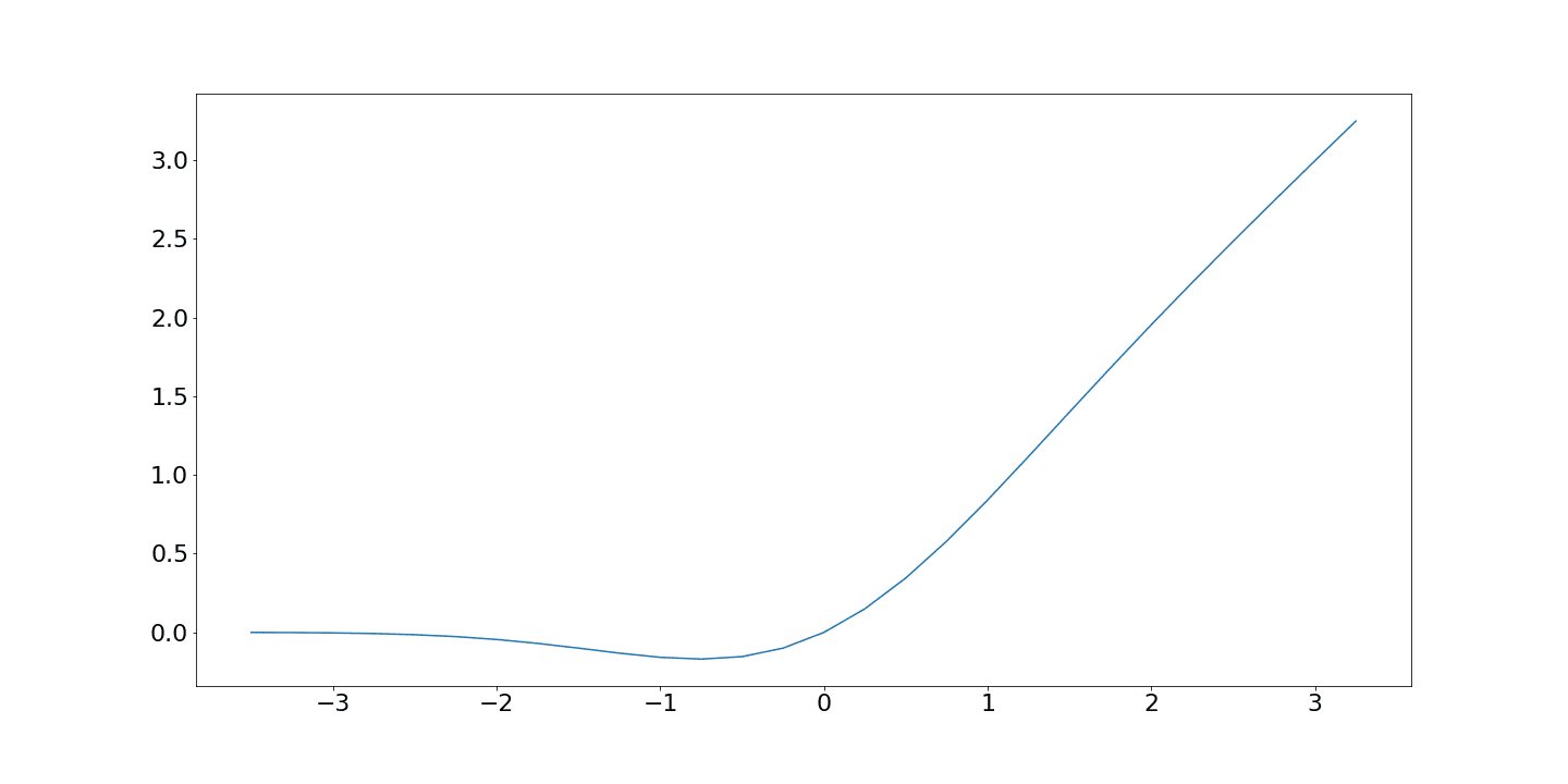
Image: GELU activation function from baeldung.com
Neuron activation calculations are matrix multiplications
When every neuron in one layer connects to every neuron in the next, computing all those outputs simultaneously can be achieved by doing a matrix multiplication. We’ll explain why here. Appendix 3 illustrates the effect that matrix multiplications achieve to help build geometric intuition.
If a layer has inputs and outputs, it requires neurons to map between them. The inputs and outputs can be arranged into vectors, and the weighted sum and bias calculation for each neuron can be represented with a matrix.
- The inputs can be arranged into a vector , a column of numbers .
- Each of the inputs (for ) is connected to each of the neurons (indexed with ) with a weight . The weights can be arranged in an matrix .
- The bias values can be arranged into a vector , a column of numbers .
- The outputs can be arranged into a vector , a column of numbers .
The weighted sum and bias calculation can be performed by multiplying the input vector by the weights and adding the biases to produce the output vector: .
So what?
This may sound abstract, but it’s just a convenient shorthand for the calculation. And it’s useful because matrix multiplications can be performed extremely quickly by modern hardware, particularly GPUs. The enormous compute cost of training and running large models is almost entirely the cost of these multiplications, repeated across billions of weights and millions of examples.
Training a neural network
A neural network starts with random weights. Training is the process of adjusting those weights so the network produces the right outputs for a given set of inputs.
Forward pass and loss
Given a training example (an input vector ), the network processes it layer by layer to produce a prediction . This is called the forward pass. The prediction is then compared to the correct answer using a loss function, which produces a single number representing how wrong the network was. Lower loss means a better prediction.
For a classification task (e.g. what animal is in an image), a common choice is cross-entropy loss, which penalises confident wrong answers heavily and rewards confident correct ones.
Backpropagation
To improve the network, we need to know how much each weight contributed to the error. This is computed via backpropagation: working backwards through the network from the loss, using the chain rule from calculus to calculate the gradient of the loss with respect to each weight.
The gradient tells us two things: in which direction a weight should be changed to reduce the loss, and roughly by how much. This is why the nonlinear activation functions used in practice must be differentiable everywhere. A function with discontinuities breaks the chain of gradients and makes backpropagation unreliable.
Gradient descent
Once we have the gradients, we update every weight by a small step in the direction that reduces the loss. This is called gradient descent:
where is the loss, is the partial derivative of with respect to (the rate of change of as is changed) and (eta) is the learning rate, a small number controlling the step size. If the learning rate is too large, updates will overshoot; too small, and training is impractically slow.
In practice, this update is not computed over the entire training dataset at once. Instead, weights are updated using small random subsets called mini-batches. This variant is called stochastic gradient descent (SGD). It is noisier but far more computationally tractable, and the noise can actually help the model escape poor solutions.
The training loop
Training repeats this cycle many times:
- Sample a mini-batch of training examples.
- Run the forward pass to compute predictions and loss.
- Run backpropagation to compute gradients.
- Update weights via gradient descent.
One full pass through the training data is called an epoch. Smaller networks are typically trained for many epochs, until the loss stops improving meaningfully. Large language models are the exception: their corpus is so large that they often see it just once, since repeating data risks memorisation instead of generalisation.
Overfitting
A model with enough parameters can memorise its specific training data rather than learning generalisable patterns. This is called overfitting: the model performs well on training examples but poorly on anything new.
Common mitigations include dropout (randomly disabling neurons during training to prevent co-dependence), weight decay (penalising large weights), and holding out a validation set to monitor performance on unseen data throughout training.
Appendix 3: Matrix multiplication illustrated
Matrix multiplication follows a simple algorithm. The result of multiplying vector by matrix is defined in two dimensions as:
This performs what is called a linear transformation. “Linear” means each output component is a weighted sum of the input components: each input contributes a term for some constant , with no squares, products, or higher powers of the inputs involved.
We can get a feel for what calculating a matrix multiplication achieves in practice by looking at some examples of the linear transformations it performs. Multiplication of vectors with more dimensions is a straightforward extension of this and what follows gives a good mental model even for vectors with many thousand dimensions, as is typical in LLM internals.
In each diagram below, the dashed arrow shows the original vector and the solid arrow shows the result after transformation. The matrix multiplication used is shown above each diagram.
Example 1: Rotation anti-clockwise by 45°
For a rotation by angle (theta) anti-clockwise, the rotation matrix is:
For , , giving:
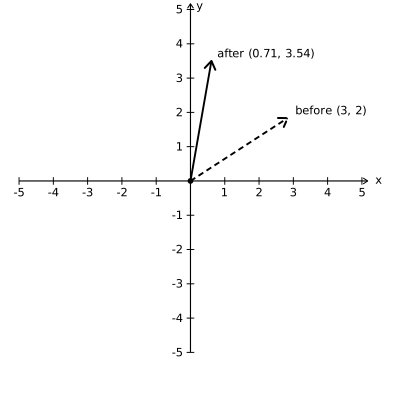
Example 2: Scaling by 1.5
Uniform scaling by factor multiplies both components by using a diagonal matrix:
The vector points in exactly the same direction but is 1.5 times longer. Notice that scaling is a special case: the before and after arrows are collinear.
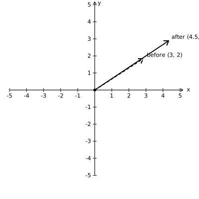
Example 3: Multiplying by −1
Multiplying by negates both components, which is equivalent to rotation by 180°:
The result is a point reflection through the origin: the vector flips to point in the opposite direction with the same magnitude.
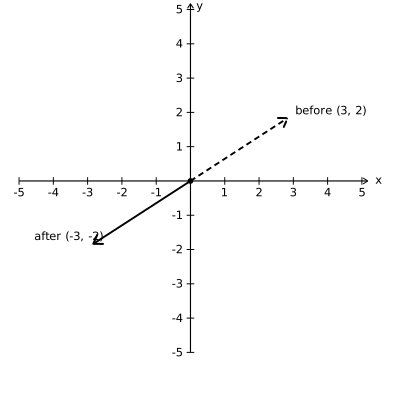
Example 4: Reflection in the line x=y
Swapping the and components reflects the vector across the diagonal line :
The two vectors are mirror images of each other across the dashed line.
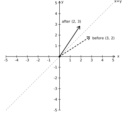
Combining transformations
A single matrix can encode a mix of these and other linear transformations, all applied in one multiplication. For example, a matrix might rotate, scale, and shear a vector simultaneously. This is one reason matrix multiplication is so useful: however complex the combined transformation, it always reduces to a single operation on the vector.
Find this useful?
We can help you apply these ideas in your workplace. Get in touch to find out how.